Principal Component Analysis : A dimensionality reduction technique

Let us try to visualize a data point or a vector in 2-dimensional space and this would be a cakewalk. Let us try to visualize the same data point or vector in 3-dimensional space; even this is fairly easy for those who are into data science. Now, let us try to imagine the same data point or vector in a 4-dimensional space. Ohh! This is where the issue starts. It is not possible to imagine a 4-dimensional space or a 5-dimensional space or in a general overview, I can state that it is quite impossible to imagine anything in an n-dimensional space while n >3. Hence, there rises the need to reduce the dimensions and we turn towards a terminology - ‘Dimensionality reduction.

So, what is Dimensionality reduction?

Dimensionality reduction is a process in which a d-dimensional data set is reduced to a d’ dimensional space such that d’<d.

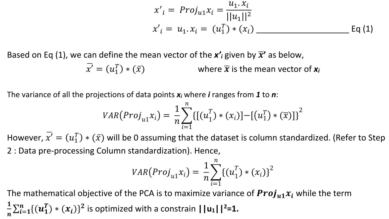
Principal Component Analysis (PCA) is one such dimensionality reduction technique where we reduce the number of dimensions involved while we still preserve the maximum variance contributed by all the involved dimensions.

Going forward, we will understand PCA as a statistical approach to visualize high-dimensional data in a 2-dimensional space and to achieve a d’-dimensional space from a d-dimensional space such that d’ is less than d for machine learning applications.

It is always easier to understand the geometric interpretation for a simple problem like 2D to 1D conversion and then we can put our understanding under the wheel to explain complex problems.

GEOMETRIC INTERPRETATION OF PCA

Let us look at a simple application of reducing 2D to 1 principal component dimension. Assume 2 different datasets which are defined by 2 dimensions i.e., Feature 1 and Feature 2 as shown below,

Let me try to interpret both FIGURE-1 and FIGURE-2 individually by conceptualizing the PCA to reduce a 2-dimensional space to a 1-dimensional space.

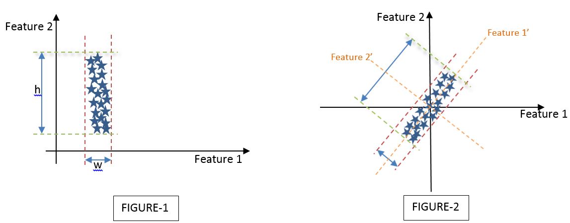
Interpretation of FIGURE-1:
We have assumed a dataset defined by Feature 1 and Feature 2 such that the variance of the dataset is the least described across the Feature 1 axis and the maximum described across the Feature 2 axis. If ‘h’ is the variance of the data set across the Feature 2 axis (i.e., Variance of the Feature 2 vector) and ‘w’ is the variance of the dataset across the Feature 1 axis (i.e., Variance of the Feature 1 vector), then by looking at the dataset I can state h>>w.

On a visual basis, and with the fact that h>>w, I can arguably state that I can discard Feature 1 and keep only Feature 2 as the principal component that describes the maximum variance of the whole dataset.

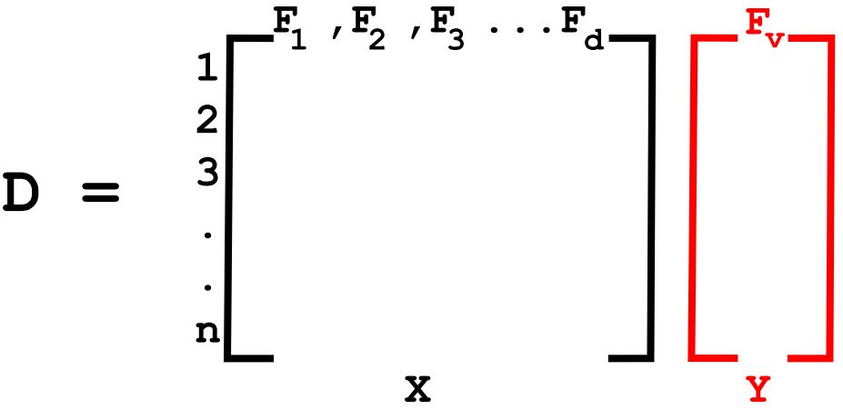
Interpretation of FIGURE-2:
However, the above is not the case in all instances and hence rises a need to explain a dataset as shown in FIGURE-2 wherein both Feature 1 and Feature 2 describe the variance of the dataset by a considerable significance. In this case, we have to describe a new axis set of Feature 1’ and Feature 2’ which is the same as the original Feature 1 and Feature 2 axis set but turned by a specific angle(Ѳ) such that the maximum variance is described along either Feature 1’ or Feature 2’ axes. In the current case, the maximum variance is described along Feature 1’s axis. Hence, we can select Feature 1’ as our principal component and proceed further either to visualize or to pipeline our machine-learning model.

MATHEMATICAL OBJECTIVE FUNCTION

Let us assume a dataset D given by {X, Y} where,
X is a random independent variable with ‘d’- features and ‘n’-data points and each data point is given by x_i where x_i ϵ R^d, a real space of d-dimensions.
Y is the dependent variable/target vector.

X alone can be represented as,

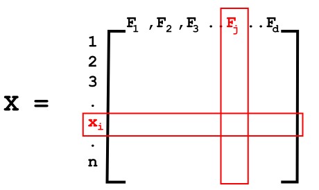
n - Number of rows meaning the number of data points (x₁, x₂, x₃...x_n)
d - Number of columns meaning the number of features (F₁,F₂,F₃....F_d)

Based on the interpretation of FIGURE-2, the objective of the PCA can be defined as finding a principal component axis (Feature 1’) on which the maximum variance of the whole dataset can be described.

Let us consider a unit vector u₁ in the direction of such principal component axis F₁'.

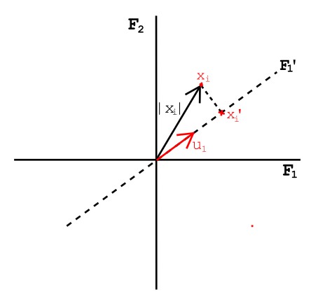
Given any point x_i in a d-dimensional space projected onto the direction of the unit vector u₁ and can be represented as,

STEPS IN DETERMINING PRINCIPAL COMPONENTS
Let us define an empirical strategy to arrive at d’ principal component axis/axes for a given d-dimensional dataset. The process would involve the below steps to arrive at the required number of principal components.

1. Data pre-processing: Column Standardization
2. Build Covariance matrix for pre-processed data set
3. Calculate Eigen values and vectors for the covariance matrix
4. Choose the principal component axes
   

Let us look at each of these steps in detail.

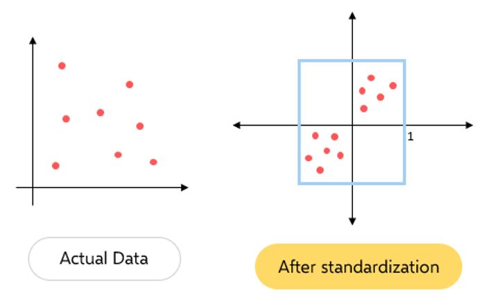
1. Data pre-processing: Column Standardization
Column standardization also known as Mean centering is a technique of scaling down any given distribution to a distribution with mean=0 and standard deviation=1.

This can be achieved by applying the below equation to each data point of the feature column:

x_ij = [x_ij - mean_j] / Standard Deviation_j

NOTE: Each feature column has to be standardized individually.

2. Build Covariance matrix for pre-processed data set
The covariance matrix can be given as matrix S of size d*d given that each element S_ij is the covariance between feature, F_i and feature, F_j of the variable X.
Hence, Covariance Matrix is given as,

S = (1/n) * X^T. X

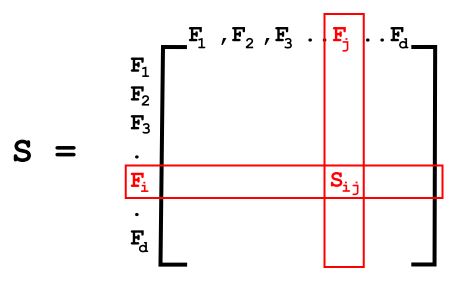
where each element is given by,

S_ij=COV(F_i, F_j)

3. Calculate Eigen Values and Eigenvectors
Eigen vectors and Eigen values are the constructs of linear algebra that are to be computed from our covariance matrix.

Eigenvectors are those whose direction does not change upon performing linear transformation and Eigenvalues are the corresponding scalar entity of each of the Eigenvectors.

In other terms, Eigenvectors are those vectors that undergo pure scaling without any rotation and the scaling factor is called the Eigenvalue.

The definition of Eigen vectors and Eigen values can be given as,

S. ν = λ. ν
where,
S – Covariance matrix
ν – Eigenvector
λ – Eigenvalue(Scalar value)

4. Choose the Principal Components
Since our covariance matrix S is a (d*d) matrix we will get d-eigenvalues and d-eigenvectors respectively.
Eigenvalues – λ₁, λ₂, λ₃..... λ_d
Eigenvectors – V₁, V₂, V₃... V_d
We arrange these eigenvalues in ascending order (λ₁>λ₂> λ₃..... >λ_d):

Principal Component 1: The eigenvector V₁ corresponding to the maximal eigenvalue(λ₁) gives the first Principal Component.

Principal Component 2: The eigenvector V₂ corresponding to the maximal eigenvalue (λ₂) gives the second Principal Component...and so on.

Intuitively the Eigenvector corresponding to the highest Eigen value represents the direction of unit vector u1 we assumed while establishing the mathematical objective function of the PCA.

And now because of PCA, we are able to reduce any random variable X of d-dimensions to d’-dimensions such that d’<d.

LIMITATIONS OF PCA

1. Loss of variance can be considerably large: While we try capturing the maximum possible variance by computing principal components, the variance or information lost across the non-principal axes could be considerably high.
2. Difficulty in interpreting Principal components: Each principal component is a linear combination of features and not a set of just important features. Hence, it is hard to interpret if a given feature is important for the given dataset.