Exploratory Data Analysis

Exploratory Data Analysis (EDA)

Exploratory Data Analysis, or EDA, is the critical first step in any data science or analytics project. It’s where we begin to dig into the dataset—cleaning it up, making sense of it, and uncovering trends or patterns that might guide future analysis. Think of it as getting to know your data before diving into complex models or predictions.

At its core, EDA is about understanding your dataset—its structure, quality, distribution, and the relationships between variables.

Let’s walk through the main stages of EDA in a practical and intuitive way.

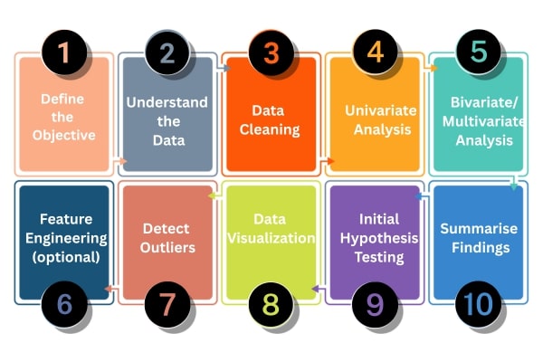
1. Define the Objective
2. Understand the Data
3. Data Cleaning
4. Univariate Analysis
5. Bivariate / Multivariate Analysis
6. Feature Engineering (optional)
7. Detect Outliers
8. Data Visualization
9. Initial Hypothesis Testing (optional)
10. Summarize Findings

1. Define the Objective

This is the first step in the eda that includes clearly stating the purpose of analysis and in simple terms defining the objective means clarifying the "why" behind your data exploration. It's about pinpointing the specific question you aim to answer or the particular problem you're trying to understand or solve using the data.
This first step is very important because it gives you a clear goal. Without knowing what you're trying to find, your analysis can become row and unhelpful. It's like asking a question or deciding what you're looking for before you start exploring the data.

2. Understand the Data

This second step involves getting familiar with the dataset itself. You need to understand its structure, the meaning of each variable, the data types, and potential sources of the data. Basically this process will call Data profiling, data reading, data viewing, this includes things like what is the size of given data,shape of the data(how many rows and columns) and what are the columns and their information and what data type of each column in a simple way to review all about data.

Details in Brief:

• Data Source: Where did the data come from? (e.g., database, CSV file, API).
• Data Structure: How is the data organized? (e.g., rows and columns, tables).
• Variables (Features): What does each column represent? What are their units (if applicable)?
• Data Types: What kind of data does each variable hold? (e.g., numerical, categorical, date/time).
• Sample Size: How many data points (rows) are there?
• Initial Exploration: Use functions like head(), tail(), info(), describe() to get a first look at the data.

3. Data Cleaning

Real-world data is often messy. This step involves identifying and handling issues that could affect your analysis. In a simple way raw data collected from domains would be incorrect and inoperable and possible reasons could be mistyping, corruption, duplication, missing values and so on. And the basic data cleaning has to be exercised before exercising any further steps of data pre-processing.

Details in Brief:

• Missing Values: Identify and decide how to handle missing data (e.g., imputation, removal).
• Duplicate Records: Detect and remove any duplicate entries.
• Inconsistent Formatting: Standardize data formats (e.g., date formats, text case).
• Incorrect Data Types: Convert variables to the appropriate data types.
• Handling Special Characters or Errors: Address any unusual or erroneous entries.

4. Univariate Analysis

Univariate Analysis is all about analyzing a single variable at a time. It helps to understand the basic features of the data, like its distribution, central tendency, and spread.

Details in Brief:

• Numerical Variables: Calculate descriptive statistics (mean, median, mode, standard deviation, quartiles, range). Visualize the distribution using histograms, box plots, density plots.
• Categorical Variables: Calculate frequency counts and percentages for each category. Visualize the distribution using bar charts or pie charts.
• Identify Potential Issues: Look for unusual distributions, skewness, or potential outliers within individual variables.

5. Bivariate / Multivariate Analysis

This step tells the relationships between two or more variables. The goal is to understand how variables interact with each other.

Details in Brief:

• Numerical vs. Numerical: Use scatter plots to visualize the relationship. Calculate correlation coefficients (e.g., Pearson, Spearman) to quantify the linear or monotonic relationship.
• Categorical vs. Categorical: Use contingency tables (cross-tabulations) to examine the relationship. Perform chi-squared tests to assess independence. Visualize using stacked bar charts or grouped bar charts.
• Numerical vs. Categorical: Compare the distribution of the numerical variable across different categories using box plots, violin plots, or by calculating summary statistics for each group. Perform t-tests or ANOVA to assess significant differences in means.
• Multivariate Analysis: Explore relationships among more than two variables using techniques like pair plots, correlation matrices (heatmaps), or dimensionality reduction techniques (if needed for visualization).

6. Feature Engineering (Optional)

This step involves creating new features from existing ones to potentially improve the performance of a model or reveal hidden patterns. It's not always necessary but can be very valuable.

Details in Brief:

• Creating Interaction Terms: Combining two or more variables (e.g., multiplying them).
• Polynomial Features: Creating higher-order terms of existing numerical features.
• Binning/Discretization: Converting numerical variables into categorical bins.
• Encoding Categorical Variables: Converting categorical variables into numerical representations (e.g., one-hot encoding, label encoding).
• Extracting Information: Deriving new features from existing ones (e.g., extracting day of the week from a date variable).

7. Detect Outliers

Outliers are data points that significantly deviate from the rest of the data. Identifying and handling them is important as they can skew statistical analyses and model performance.

Details in Brief:

• Visual Methods: Use box plots, scatter plots to visually identify potential outliers.
• Statistical Methods: Use techniques like the IQR method (Interquartile Range), Z-score, or DBSCAN algorithm to detect outliers based on statistical properties.
• Handling Outliers: Decide how to treat outliers (e.g., removal, transformation, capping, or keeping them if they represent genuine extreme values).

8. Data Visualization

Visualizations are essential for understanding patterns, trends, and relationships in the data. They make complex information more accessible and help in communicating findings.

Details in Brief:

• Choosing Appropriate Plots: Select visualization techniques that are suitable for the type of data and the relationship you want to explore (e.g., histograms for distributions, scatter plots for correlations, bar charts for comparisons).
• Creating Clear and Informative Visuals: Ensure plots have clear labels, titles, legends, and are easy to interpret.
• Exploring Different Perspectives: Create multiple visualizations to look at the data from various angles.

9. Initial Hypothesis Testing (Optional)

Based on the initial observations and patterns, you might want to perform preliminary statistical tests to formally assess certain hypotheses.

Details in Brief:

• Formulating Hypotheses: State specific claims about the data that you want to test.
• Choosing Appropriate Tests: Select statistical tests based on the type of data and the hypothesis being tested (e.g., t-tests for comparing means, chi-squared tests for independence).
• Interpreting Results: Understand the p-values and make initial inferences about the hypotheses. This step can guide further, more formal statistical analysis.

10. Summarize Findings

After performing the analysis, it's crucial to synthesize your observations and insights into a clear and concise summary.

Details in Brief:

• Key Patterns and Trends: Highlight the most important relationships, distributions, and anomalies you discovered.
• Answering the Initial Objective: Relate your findings back to the original question or problem you set out to address.
• Limitations of the Analysis: Acknowledge any limitations in the data or the analysis performed.
• Recommendations or Next Steps: Suggest potential further investigations, modeling approaches, or actions based on your findings.

Overall, the goal of EDA is to gain a better understanding of the data and to identify potential hypotheses or questions that can be further tested and explored. By using visualization and statistical analysis, you can better position yourself to make informed decisions and draw accurate conclusions about your data.