Hypothesis Testing in Datatab

I have always wondered what goes inside the heads of these statisticians who live and Breathe hypothesis and its testing.

t’s funny how they first decide to assume things, build a hypothesis and then try their level best to find witnesses to discard it.

So, in the end, all they do is contradict their own theories?

Well in today’s blog I am going to introduce to you the concept of hypothesis testing. And the irony? Well in the end, either you will reject or fail to reject your own hypothesis.

Wait for it!

So let me begin by introducing to you “The Stats Family”

We have two brothers Mr. Hypothesis Stats, the elder one, and Mr. Inference Stats, the younger one. They have two dogs, Alpha and Beta. They are very close to their two grandmothers, Independent Sample Nanny and Dependent Sample Nanny. I know you must be wondering what weird names these are, (trust me I have been thinking the same about the entire hypothesis testing but who are we to judge) so just hang in there, it will all start to make sense in some time…hopefully! The bigger game is that of inferential statistics under which, hypothesis testing is a subset. We usually tend to use hypothesis tests to draw inferences out of sample data and estimate the accuracy of the inference on population data. I will today introduce you to the basic understanding of hypothesis testing using a case study on a web application tool – DataTab https://datatab.net/

DataTab.net is one of the most simple to use statistical apps that can perform the most advanced statistical analysis. So you definitely will enjoy using the tool.

First and foremost, what is hypothesis testing, and how is it conducted?

To give you a basic idea, Mr. Hypothesis Stats works hard every day so that in the end he can come back home and give his greatest learnings of the day to his younger brother Mr. Inference Stats. He sometimes takes Inference to Independent Nanny’s home and sometimes to the dependent Nanny’s home. Without any bias, both these kids love their two grandmothers equally. However, They prefer dog beta to dog alpha while going to their nanny’s house because beta is well-behaved and alpha on the other hand bites ferociously. Read on and you will learn why and the story will start making sense!

Road Map for Inferential statistics.

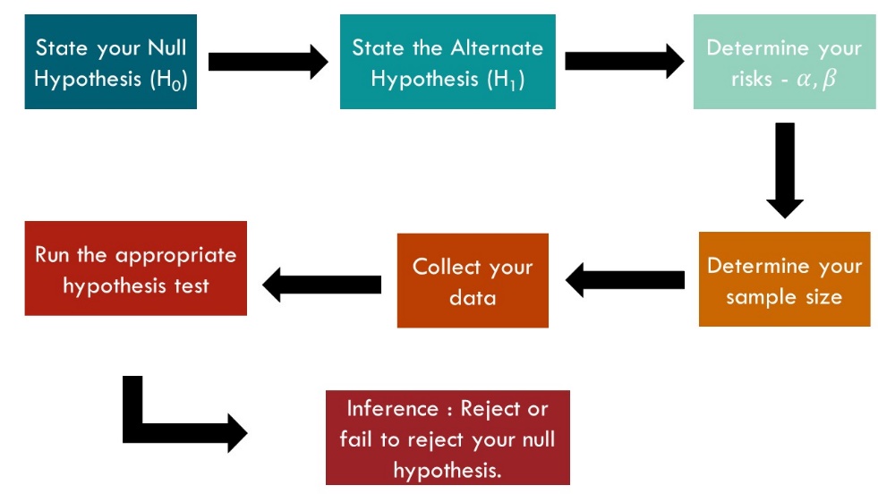
Step 1: We begin by assuming a statement called the null hypothesis (H0) which is a statement involving a population parameter. Along similar lines, we state a statement alternative to it called the alternative hypothesis (H1) which is opposite to the null hypothesis.

Step 2: One of the greatest life lessons Mr. Hypothesis has taught Mr. Inference is that every assumption involves risks and we must manage our risks in order to achieve greater success. Only if millennials would get that! Thus, whenever we draw inferences using sample data on the population, there is always a risk involved. How much are you willing to accept the risk, confidence level of 99%, 95% or 90%. With the level of risk, one is ready to take, we set the level of significance which can be 0.01 or 0.05 or 0.1 corresponding to each confidence level.

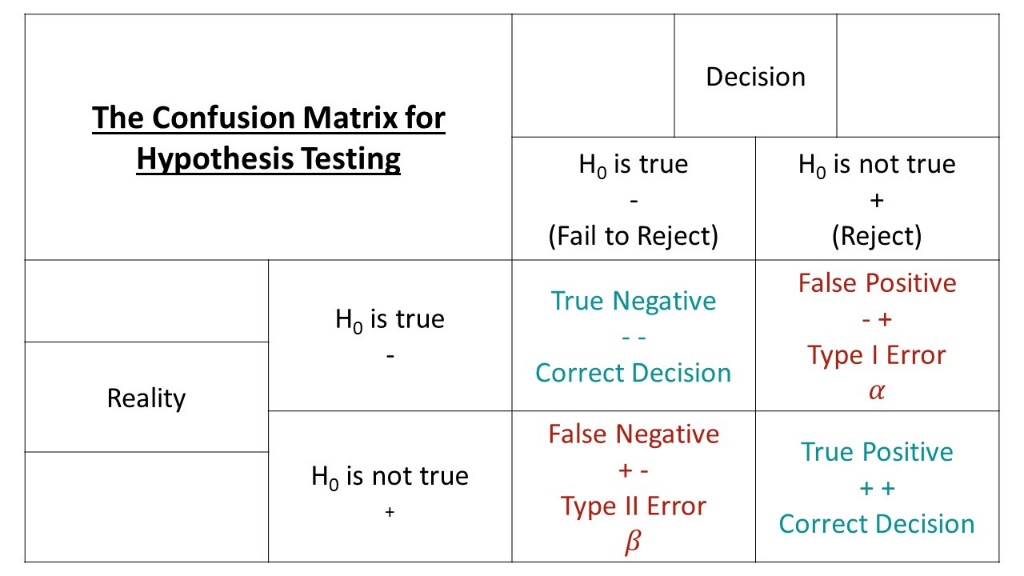
Step 3: While managing risks there can also be errors. Every hypothesis testing comes with two types of errors

Type 1 Error: alpha

You reject H0 when in reality it’s actually true! It’s unfair yes, but it happens many times. We call this kind of error an alpha error.

Type 2 Error: beta

You fail to reject H0 when you should have. We accept a hypothesis when in reality it’s actually wrong. Below is a table that can give you a concise view.

Step 4: Once the hypothesis is stated we then carry out testing based on our parameters and data in order to reject H0 or fail to reject H0. Told ya!

Step 5: Once we complete our testing, we obtain a p-value. It tells us what is the possibility of our results if we take our null hypothesis to be true. The point to note is, that the p-value also called the observed level of significance if found to be less than our chosen level of significance, we reject our null hypothesis or else we fail to reject the null hypothesis. This is the story of hypothesis testing. Apologies for the trauma you are going through but it’s a part of life now.

The story of Dependent and Independent Nanny

Dependent Nanny loves to cook and her favorite ingredient is potato. She experiments, creates, imagines, and invents the most amazing kinds of foods but keeps potatoes as the main and common ingredient like aloo-tikka and French fries. On the other hand, Independent Nanny also loves to cook, but usually, her dishes are poles apart from each other. While she might cook fish, on one hand, she would also cook rajma-chawal on the other, and while both are fantastic dishes, they absolutely hold no similarities. Drawing the analogy from here, hypothesis testing is conducted on independent and dependent samples. Two samples may be independent if they are not related to each other like fish and rajma chawal and are dependent if one sample can be used to draw estimations of other samples like aloo-Tikka and French fries. This way, depending on the type of samples we use, our approaches for hypothesis testing also vary. I know, head spins much? It's okay, Let's visualize using DataTab and understand what is happening. Kindly note that this case study only deals with the hypothesis and inference of samples and not the actual math that goes behind conducting hypothesis testing. Though studying that and learning from scratch is always recommended.

Case Study using DataTab

We will use a dataset of the mileage of different car types: hatchback, wagon, sedan, coupe, and convertible.

Inserting and checking data

In DataTab it is easy to upload a dataset by cut-copy method or by simply importing your .csv or .xsl file.

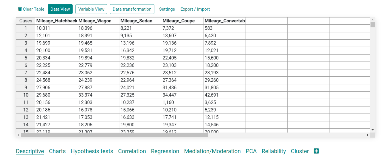
We chose two samples from this dataset, say mileage of hatchback and mileage of wagon.

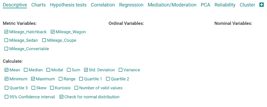
Let us first visualize in order to determine whether both these samples are normally distributed in order to decide which test to perform

DataTab allows us to choose our samples and plot different properties together.

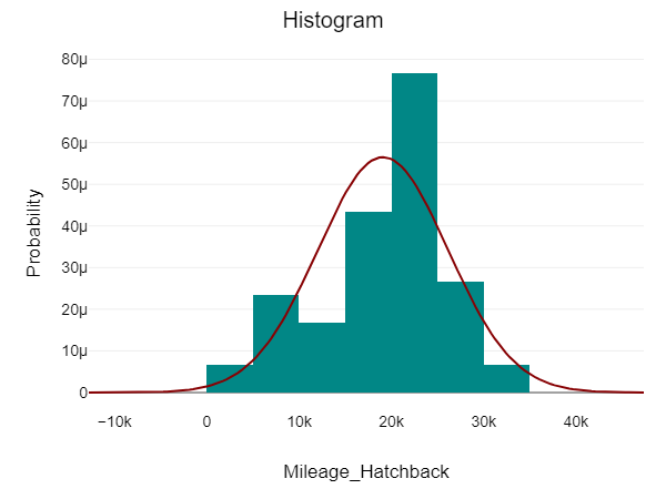
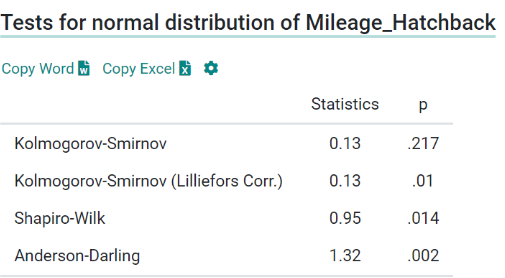
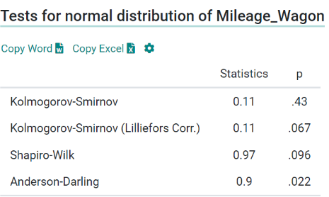
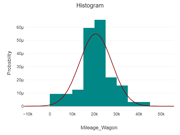
For both these samples, the data points (n) are greater than 50. Thus we follow the Kolmogorov-Smirnov test to test their normality. Kolmogorov-Smirnov Test is a non-parametric test that assumes a null hypothesis that the sample comes from a normal distribution. If the p-value > 0.05 then the hypothesis is retained and the sample is said to be in a normal distribution. Here for both samples, the p-values are 0.217 and 0.43 respectively. Thus, our samples are normally distributed and we can go ahead with our hypothesis testing. Now, that both our samples are in normal distribution and sample size > 50, hence we can conduct the t-test for hypothesis testing.

t-test

Step1: Set desired parameters In DataTab, conducting a t-test is just a matter of a few clicks.

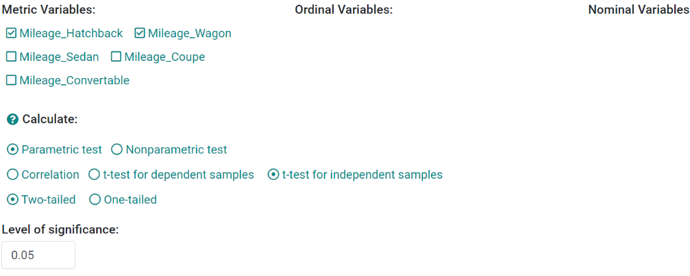
We chose two samples: Mileage_Hatchback and Mileage_Wagon. We have to perform a parametric test which is a t-test for two independent samples.

Note: Our t-test will be two-tailed. We also select the level of significance as 0.05.

Step 2: Draw null and alternative hypothesis

DataTab is an intelligent software that draws both null and alternative hypotheses on its own for the user.

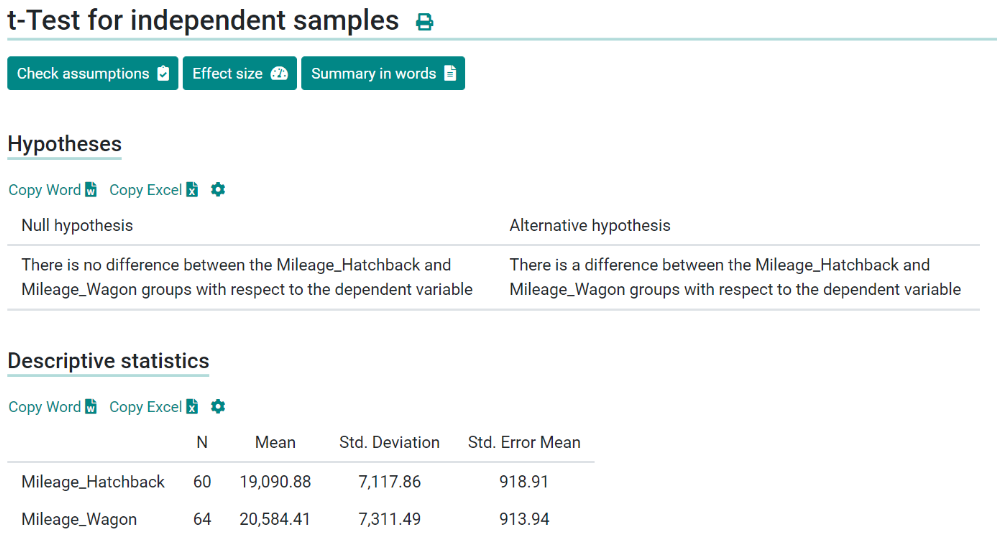
Null Hypothesis: There is no difference between the Mileage_Hatchback and Mileage Wagon groups with respect to the dependent variables.

Alternative Hypothesis: There is a difference between the Mileage_Hatchback and Mileage Wagon groups with respect to the dependent variables.

Also, note the standard deviations of the two samples are relatively closer/similar to one another.

Step 3: Conduct the t-test

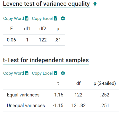
With equal variances, the p-value obtained for our t-test is 0.252. p-value > level of significance (0.05) Therefore, we fail to reject our null hypothesis, and thus it is retained.

One of the most helpful features of DataTab is that it provides a summary of tests which can then be used directly in any kind of research work and projects.

Step4: Inference

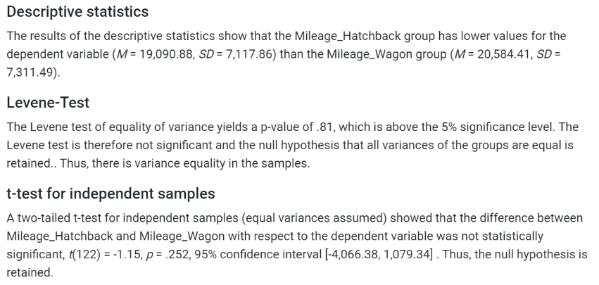
Descriptive statistics- The results of the descriptive statistics show that the Mileage_Hatchback group has lower values for the dependent variable (M = 19,090.88, SD = 7,117.86) than the Mileage_Wagon group (M = 20,584.41, SD = 7,311.49).

Levene-Test- The Levene test of equality of variance yields a p-value of .81, which is above the 5% significance level. The Levene test is therefore not significant and the null hypothesis that all variances of the groups are equal is retained. Thus, there is variance equality in the samples.

t-test for independent samples- A two-tailed t-test for independent samples (equal variances assumed) showed that the difference between Mileage_Wagon with respect to the dependent variable was not statistically significant, t(122) = -1.15, p = 0.252, 95% confidence interval [-4,066.38, 1,079.34] .

Thus, the null hypothesis is retained.